Motivation
Cloth simulations are EVERYWHERE. They show up in gaming, AR/VR, robotic manipulation, digital fashion, even synthetic data generation for training VLMs. But cloth dynamics aren't just about visuals anymore, but also about bridging perception and physics and enabling robots to handle deformable objects precisely.
Enter: Differentiable simulators. They work on the idea that your physics engine doesn't need to be treated like a black box. Instead, make it fully differentiable so you can optimize physical parameters using gradient descent.
The Math Behind Differentiable Simulators
It starts with an initial guess for physical parameters \(\theta\) (mass, friction, stiffness, geometry, etc.). The differentiable physics engine simulates motion and deformation frame-by-frame, giving you object states at each timestep: positions, velocities, mesh vertices.
These states get passed into the differentiable renderer, which produces rendered video frames from the simulated scene. These rendered frames are compared to the ground truth video using pixel-level loss.
Backpropagate that error through both the renderer and the physics engine simultaneously. The gradients flow back to \(\theta\), giving you \(\partial L / \partial \theta\) which corresponds to the exact sensitivity of pixel error to each physical parameter. Hence \(\theta\) updates, rinse, repeat. The only thing now that stands between the physics and the pixels is one loss function.
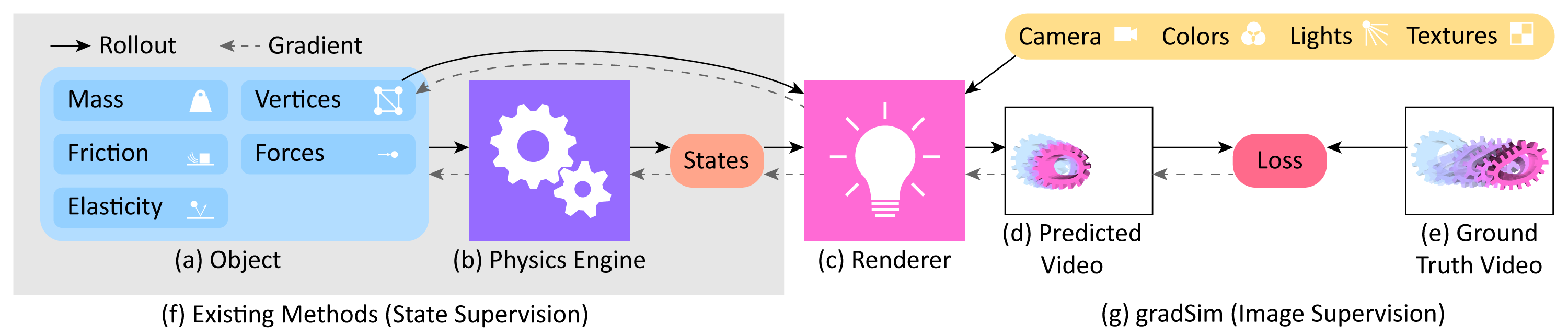
Formally, the simulation is a map:
\[ \text{Sim} : \mathbb{R}^P \times [0,1] \mapsto \mathbb{R}^{H \times W}, \quad \text{Sim}(p,\, t) = I \]where \(p \in \mathbb{R}^P\): simulation state and parameters, \(t\): simulation time, \(I\): rendered image of height \(H\) and width \(W\) at timestep \(t\).
If \(\text{Sim}\) is differentiable, then \(\nabla \text{Sim}(p, t)\) tells you how an infinitesimal perturbation \(\delta p\) changes the output — from \(I\) to \(I + \nabla \text{Sim}(p,t)\,\delta p\). This enables gradient-based optimization: define a loss \(\mathcal{L}(I,\, I_{\text{target}})\) over image space and descend along \(-\nabla \text{Sim}\) to minimize it:
\[ p^* = \arg\min_p \; \mathcal{L}\!\left(\text{Sim}(p,\, t),\; I_{\text{target}}\right) \]The Engineering Challenge
Normal renderers aren't differentiable. Pixels are discrete and triangle edges are hard. Differentiable renderers like SoftRas replace these with smooth approximations: probabilistic triangle boundaries where pixels blend as geometry moves, making \(\partial I / \partial (\text{mesh position})\) well-defined.
On the physics side, you're differentiating through an ODE integrator across 100+ timesteps. Physics is full of discontinuities. The gradient flow has to survive all of these without exploding or vanishing. That’s the hard part.
gradSim is one such open source differentiable simulator and renderer. I wanted to dig deeper into this codebase and rewriting it in JAX seemed like a lowkey fun way of going about it. In the process I also grew familiar with the JAX way of thinking about computation.
Read on for a deeper dive.
The Intuitive Difference
Frameworks encode worldviews.
PyTorch's worldview: Your code is living and breathing. Objects hold states, gradients accumulate, sprinkle backprop calls wherever it makes sense, and the computation graph builds itself as your code runs; tracking everything automatically.
JAX's worldview: Your code is just math, where functions take inputs and return outputs.
Optimizers
In PyTorch, optimizers are black boxes. You create one, call it, and your parameters update.
JAX forces you to write the optimizer yourself. At first this feels like punishment. Then you realize that the optimizer state is just data that you can inspect, save mid-training and modify the update rule on the fly. The black box we started out with turns out to be just differential equations.
"Neural Networks"
Most of the neural networks in the original codebase weren't really neural networks. They were single matrix multiplications with a tanh on top.
Porting it to JAX forces you to think about what it's actually computing. And the answer was usually a simple, straightforward weighted sum.
A weight matrix is as simple as it gets. If you genuinely need modular neural architectures, libraries like Flax exist. But the default should be: write what you want and not what the framework encourages. JAX forces you to be explicit about what you want.
Translating OOP
Physics simulations are naturally stateful. You have a model object that represents your scene — springs, masses, friction parameters. These parameters are read from the object’s state and are updated, rinse, repeat. (Standard OOP)
PyTorch handles this well because it is fundamentally Object-Oriented.
JAX on the other hand: absolutely not. Mutation inside a traced function breaks everything.
The fix: rebuild the scene configuration from parameters every forward pass. As insane as that sounds, it's simply re-specifying the configuration every forward pass, not running any physics. So, reconstructing that each time costs almost nothing.
This exposed a design smell in PyTorch: the model object smuggles three conceptually different things: Static scene topology, trainable physical parameters, and time-varying simulation state into the same data structure.
JAX separates these cleanly and makes them traceable by eye. Configuration as structure, parameters as data, state as explicit input/output. It sure made the code harder to write but also impossible to misunderstand.
Small Things That Compound
Device Management
JAX figures out device management automatically. This in PyTorch would mean constantly shuttling tensors between CPU and GPU, tracking which device each object lives on, and debugging shape mismatches that turn out to be device mismatches. This feels like a minor convenience until you add up the cumulative hours spent chasing down cuda calls that shouldn't have been necessary in the first place.
Type Strictness
PyTorch silently converts Python tuples to tensors if you try to add them. Convenient! But also: hides type mismatches that should have been errors.
JAX throws errors immediately instead of letting type mismatches silently propagate into useless gradient errors later. Annoying until it saves you from debugging sessions where the error is three function calls deep and tells you nothing.
Explicit Randomness
PyTorch has a global random state. JAX makes you thread random keys through your functions explicitly. Feels like bureaucracy until you need to reproduce a bug and realize implicit randomness is a debugging nightmare.
For my use case (physics simulation where randomness is mostly in data generation), this is mostly irrelevant, but the design choice is revealing: JAX would rather be verbose than hide state.
When PyTorch Is Actually Better
The abstractions in PyTorch are great when you're learning, or for quick experiments where the architecture changes hourly. Being able to generally treat code like an interactive notebook is powerful.
But for a differentiable physics simulator where:
- Correctness matters more than iteration speed
- You'll eventually JIT-compile everything into one GPU kernel
- Gradient flow debugging is crucial
- The code runs for hours on a cluster
you NEED JAX's enforced constraints and explicitness, rightly so.
This made me realise backpropagation much more intuitively.
You see the actual update equations and calculus' chain rule spelled out in code.
When your entire goal is computing df/dx, having 'f' actually BE a function and not an object that mutates makes everything cleaner.
If you can't express something as a pure function, you're probably dealing with something that shouldn't be differentiable in the first place.
Hence, naturally for differentiable physics, JAX's functional worldview fits perfectly.